
1. Strategy and Annotation Principles
For Stereo-seq spatial transcriptomics (ST) data, we recommend single-cell reference–based deconvolution: use known cell-type expression profiles from scRNA-seq to infer the cell-type composition of each spatial unit (bin/cellbin), and thereby reconstruct the spatial distribution of cell types.
Annotate coarse-to-fine: first assign robust major cell types, then refine selected major types into cell subtypes.
2. Single-Cell Reference Preparation
2.1 Data Sources and Selection
Prefer an in-house scRNA-seq reference from the same sample and tissue as your ST data. This minimizes batch effects and maximizes biological match.
Fall back to public or published datasets of matching tissue when in-house data are unavailable. Check provenance, sequencing platform, and tissue source to limit bias.
Useful public repositories:
CELLxGENE (CZI Science): https://cellxgene.cziscience.com/
Broad Single-Cell Portal (SCP): https://singlecell.broadinstitute.org/single_cell
2.2 Quality Control
Reference quality sets the ceiling for annotation accuracy. The references are the "benchmark" of annotation: mislabeled or missing cell types propagate directly into the ST annotation. QC before annotating is mandatory.
Standard QC: cell filtering (nFeature, nCount, mitochondrial fraction), doublet removal, etc.
Label validation: use marker-gene dotplots to confirm that each labeled cell type shows specific expression of its markers, with no obvious mislabeling or cross-contamination. The reference may be used for deconvolution only after its labels pass the marker-gene validation.
import scanpy as sc
import scrublet as scr
import numpy as np

adata = sc.read_h5ad("ref.h5ad")

# 1. Standard QC: gene/cell filtering + mitochondrial fraction
adata.var['mt'] = adata.var_names.str.startswith('MT-')   # use 'mt-' for mouse
sc.pp.calculate_qc_metrics(adata, qc_vars=['mt'], inplace=True)
sc.pp.filter_cells(adata, min_genes=200)
sc.pp.filter_genes(adata, min_cells=3)
adata = adata[adata.obs.pct_counts_mt < 20, :].copy()

# 2. Doublet removal (single-sample reference shown here).
#    For multi-sample references, run this per sample.
rate = min(0.008 * adata.n_obs / 1000, 0.25)
sc.pp.scrublet(adata, expected_doublet_rate=rate, random_state=0)
n0 = adata.n_obs
adata = adata[~adata.obs['predicted_doublet'].astype(bool)].copy()
print(f"doublets removed: {n0} -> {adata.n_obs}")

# 3. Normalize + log-transform for marker dotplots
sc.pp.normalize_total(adata, target_sum=1e4)
sc.pp.log1p(adata)
2.3 Organizing the Cell-Type Hierarchy
If the reference is already annotated at the subtype level, collapse subtypes into their major cell types before running major-type deconvolution. Major types differ sharply in expression and separate cleanly; subtypes differ subtly and are easily confused when deconvolved across a whole chip. Handle subtype refinement later, within each major type (Section 4).
3. Major Cell-Type Annotation
The core task is to pick a suitable deconvolution algorithm and apply it to the ST data to obtain the major cell-type proportions or the dominant assignment of each spatial unit. Algorithms differ in how well they handle data scale, sparsity, and tissue type.
3.1 Obtaining Tools
Option 1 — SDAS: SDAS (Stereo Data Analysis Solution) is an "out-of-the-box, unzip-and-run" Linux command-line analysis toolkit developed by BGI STOmics for Stereo-seq data. It ships an end-to-end pipeline from preprocessing to plotting and bundles four deconvolution methods — cell2location, RCTD, SPOTlight, and Tangram — so you can annotate without installing each one separately.
SDAS Download:
SDAS GitHub:
Option 2 — Official algorithm releases: Install the algorithms directly from their official repositories, following the official documentation.
3.2 Algorithm Selection
The STOmics website has benchmarked cell2location, RCTD, SPOTlight, Tangram, SCimilarity and other methods on Stereo-seq data across tissue types and resolutions, covering accuracy and resource consumption, which can serve as a reference for tool selection (we suggest considering data scale, tissue type, and other features of your data):https://www.stomics.tech/STOmicsNews/2296.html
3.3 Handling NA Results
Deconvolution can leave some bins/cells with an NA label — the unit could not be matched to any reference cell type, usually because of low quality or mixed signals. This happens at both the major-type and subtype level.
If the NA fraction is low: discard those spatial units from downstream analysis.
If the NA fraction is high: re-examine the quality of the raw ST data and the suitability of the scRNA-seq reference.
4. Cell Subtype Annotation
Subtype annotation assumes that Section 3 has produced reliable major-type labels; subtype refinement proceeds only within each major type. Core principle: each major type is extracted and subtyped independently — in both 4.1 and 4.2, first extract the spatial units belonging to one major type, then run downstream analysis on that subset only, using only that major type's subtype markers.
4.1 Gene-Set Scoring and Hierarchical Clustering
Performed separately for each major type: Extract the spatial units for one major type, then score and cluster them using that major type's subtype signature genes, fully isolated from the others. Do not pool subtype markers from all major types into one clustering run — the resulting clusters no longer align with the major-type labels, and the subtype results become disconnected from the annotation above it.
Workflow: gene-set scoring → hierarchical clustering → cluster-level subtype call → label assignment. See Section 7 for reference code.
Gene-set scoring: log-normalize the extracted expression matrix, then score every spatial unit against each subtype's signature gene set (subtype markers, or subtype DEGs computed within this major type in the scRNA-seq reference). The result is a subtype × unit score matrix.
Hierarchical clustering and assignme: hierarchically cluster the units based on the score matrix, cut the tree into many fine clusters, and assign each cluster to the subtype with the highest mean score.
Clusters without a clear subtype: if a cluster shows no strong signal for any candidate subtype, it lacks distinct subtype features but still belongs to this major type. Label such clusters <MajorType>_Other (e.g., B_Other, T_Other), not just "Other".
Validation: check the result with a marker-gene heatmap. If scoring is generally weak, the chosen signature genes lack specificity — swap them and re-run.
Reference: Tang Z, et al. Spatial transcriptomics reveals tryptophan metabolism restricting maturation of intratumoral tertiary lymphoid structures. Cancer Cell, 2025; 43, 1025–1044.e14.
4.2 Subtype Deconvolution
Performed separately for each major type: Split both the ST data and the scRNA-seq reference by major type, then deconvolve subtypes within each.
Subtype the scRNA-seq reference first: extract all cells of the major type, then subcluster and label subtypes within that subset using the standard single-cell workflow (marker-based assignment).
Extract the corresponding ST spatial units: extract all spatial units annotated as this major type from the ST data.
Deconvolve within the major type: using the subtyped single-cell subset as the reference (algorithms as in Section 3). Splitting by major type narrows the candidate set and reduces cross-type confusion, making subtypes easier to resolve.
NA results: units that fail to match any subtype still belong to this major type. Label them <MajorType>_Other (e.g., B_Other, T_Other) to preserve major-type membership.
5. Evaluating the Annotation Results
After annotation, cross-validate the reliability of the results from multiple dimensions:
Marker-gene expression heatmap: check whether the marker genes of each cell type are specifically enriched in the corresponding cell type. Plot z-scored mean expression to normalize away absolute abundance differences and make cross-gene comparison meaningful.
Deconvolution score heatmap: check whether the "dominant label" matches the deconvolution score — with accurate annotation, high values concentrate on the diagonal (code in 7.2).
Plausible proportions: check whether the inferred cell-type proportions are within a reasonable range compared with the scRNA-seq reference and known tissue composition.
Consistency with the reference: check whether the cell-type composition and expression profiles of the ST annotation match the scRNA-seq reference (code in 7.3).
Histology (H&E) alignment: compare the annotated regions with histological morphology and confirm consistency with anatomical structures (e.g., cortex, glands, stromal regions).
If results are unsatisfactory, trace back through the pipeline — reference quality, algorithm choice, parameters, bin size — and isolate the source of the problem.
6. Special Cases: Tiled / TMA Samples
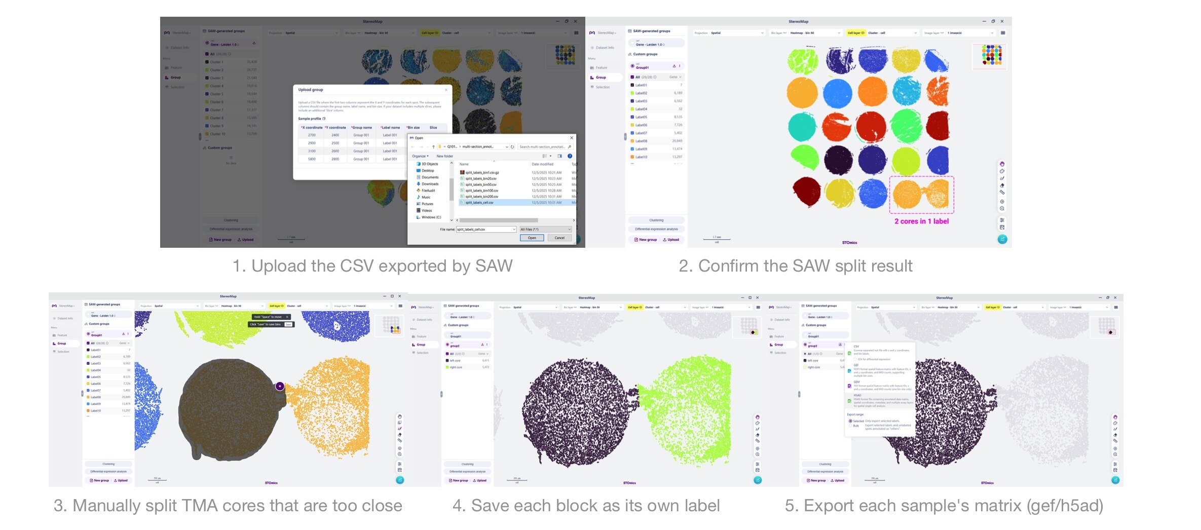
For tiled samples and tissue microarray (TMA) samples, whole-chip annotation may perform poorly when inter-sample batch effects or tissue heterogeneity are strong. In that case, we suggest annotating sample independently and then merging the results. Per-sample annotation reduces cross-sample interference and improves accuracy.
To split a tiled or TMA samples, the recommended approach is SAW count or SAW realign (≥ 8.3.0) with the --split-tissue-into-labels parameter . If your data were generated with an older SAW (< 8.3.0) and re-running is impractical, you may split it manually with a Python script based on the tissue mask already exported by SAW.
6.1 Splitting with SAW (Recommended)
Run SAW count or SAW realign (≥ 8.3.0) with --split-tissue-into-labels parameter. SAW automatically identifies each tissue block from the image and assigns it an independent label region. Load the output into StereoMap (≥ 4.3.0) to review and adjust the labels visually, then export a per-block gef/h5ad for downstream analysis.
SAW 8.3.0 documentation: https://www.stomics.tech/service/new-saw-operation-manual.html
StereoMap 4.3.0 documentation: https://www.stomics.tech/service/new-StereoMap.html
6.2 Manual Splitting from the Tissue Mask
This Python script takes the h5ad file and the tissue mask exported by SAW and returns an h5ad with a per-unit obs['mask_label']:
import scanpy as sc
import cv2
# tissue mask: result/sample/outs/image/sample_ssDNA_tissue_cut.tif

def split_tma(h5ad_file, tissuemask):
    adata = sc.read(h5ad_file)
    adata.X = adata.raw.X    # optional: swap in the raw expression matrix if needed
    mask = cv2.imread(tissuemask, cv2.IMREAD_GRAYSCALE)
    num_labels, labels = cv2.connectedComponents(mask)
    label_list = []
    for i in adata.obs.iterrows():
        cx = i[1]['x']
        cy = i[1]['y']
        this_label = labels[cy, cx]
        label_list.append(this_label)
    adata.obs['mask_label'] = np.array(label_list).astype(str)
    return adata

adata = split_tma("sample.h5ad", "outs/image/sample_ssDNA_tissue_cut.tif")
# Inspect the spatial distribution of the labels
sc.pl.spatial(adata, color='mask_label', spot_size=20, show=False, legend_loc="on data")
Reference Code
Cell subtype hierarchical clustering:
http://cdn-newfile.stomics.tech/software-packages/celltype_annotation/anno_score_heatmap.ipynb
Deconvolution score heatmap:
http://cdn-newfile.stomics.tech/software-packages/celltype_annotation/hier_clustering_subtype.ipynb
Consistency analysis with reference cell types:
http://cdn-newfile.stomics.tech/software-packages/celltype_annotation/metaneighbor_correlation.ipynb